
For this blog entry, I'll be discussing Fourier transform. For those who do not know anything about Fourier Transform (FT), just imagine that it's a way to a new world—in this world, you see frequency profiles instead of the usual things you see.
In this world, which is called the Fourier domain, you can remove (or add) details that are repetitive in the ‘real’ world. For example, if there are 5 equally spaced ball pens on a table, if you go to the ‘Fourier World’, you can see this as peaks. These peaks can be removed and when you go back to the ‘real world’, the ball pens will be gone, leaving you with the table.
To get you started, we first want to be familiar with how this Fourier thing goes. Figure 1 shows different Fourier transforms of different image patterns. We generated a circle, an annulus, a square, a horizontal double slit, a vertical double slit and two dirac deltas symmetric with the y-axis.
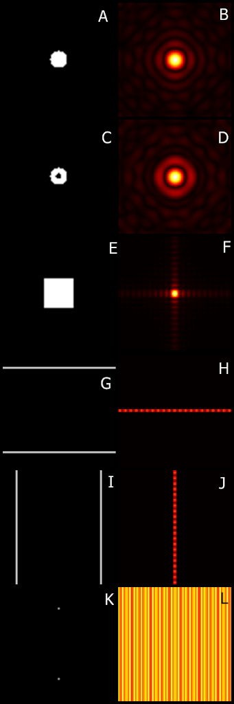
Figure 1. Different image patterns: (a) circle, (c) annulus, (e) square, (g) horizontal double slit, (i) vertical double slit and (k) two dirac deltas symmetric with the y-axis and their corresponding Fourier transforms (b, d, f, h, j and l, respectively).
The circle and the annulus have a similar Fourier Transform, which are both circular in nature. The square has a square-ish FT which is indicative of its shape. More shapes (or apertures in this case) have unique FTs. Next are the FTs of the slits. Again, both FTs are indicative of their original image. Last is the FT of two dots symmetric along the y-axis. We can see that it has a somewhat sinusoidal pattern along the x-direction.
Note that we may be exchanging the terms FT and FFT. FT means Fourier Transform while FFT means Fast Fourier Transform. The main difference is, well, the latter is, uhm, fast. Yeah, I'm not joking! FFT uses 2^x where x is a number to optimize FT, making it fast. Most programs use FFT to save time instead of directly evaluating FT by itself. :)
For the next part of the activity, we were asked to find the FT of two dirac deltas, two circles and two squares. The dots show a fan-like FT with sinusoidal ridges. As for the circles, it is similar to the FT in Figure 1b. Conversely, the FFT of the squares is similar to that of Figure 1f. This is again because certain apertures have a unique corresponding FFT pattern.
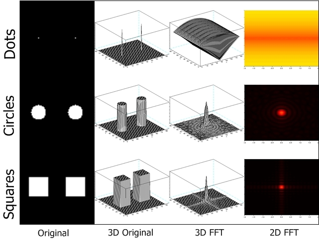
Figure 2. The 3D rendering of two dots, circles and squares with their corresponding FFT in 2D and 3D.
Next we try to examine the effect of varying the variance of a Gaussian function. What we can conclude is that the larger the variance, the smaller its FFT.
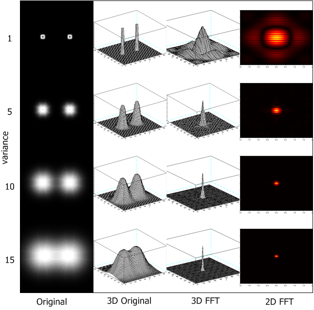
Figure 3. The 2D and 3D FFT of Gaussian functions in increasing variance.
Now, we create a 200×200 matrix of zeroes with 10 points at random with values of 1. These will be the deltas. This is called array A. We also make a 200×200 matrix with a single pattern at the middle. This one shall be called array d. We then convolve the two by taking the Fourier Transform of both A and d, multiplying them element-per-element then taking the inverse Fourier transform. We tried it with three types of patterns: a cross (within the 5×5 pattern in the manual), an arbitrary cute shape which is larger (to try out what happens if we do not use a 5×5 pattern) and a large circle (to go to the extreme!). What just happened is at the points where there is 1, the pattern is replicated. Check out the convolution when using the large circle; it may even be used for a wallpaper. 😄
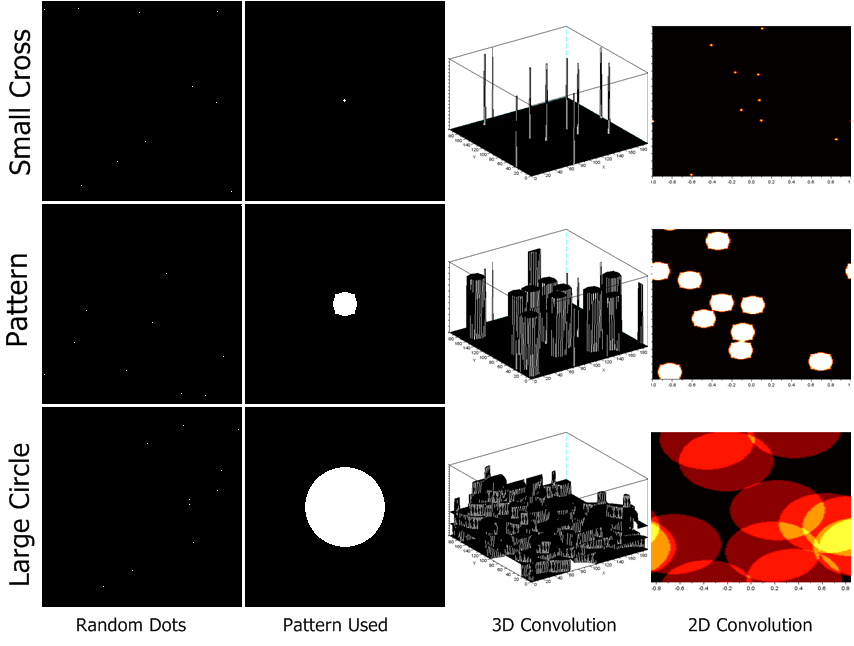
Figure 4. Convolution of two images. The random dots are convoluted with a certain pattern. The resulting convolution is shown in 2D and 3D.
Next we try to examine the effect of pixel spacing in images. We used a 200×200 array with equally spaced 1s. We get the FT of each. As you can see, when the spacing of the dots is smaller, the peaks in the FT are few. As the spacing of the dots increases, the number of peaks in the FT also increases.
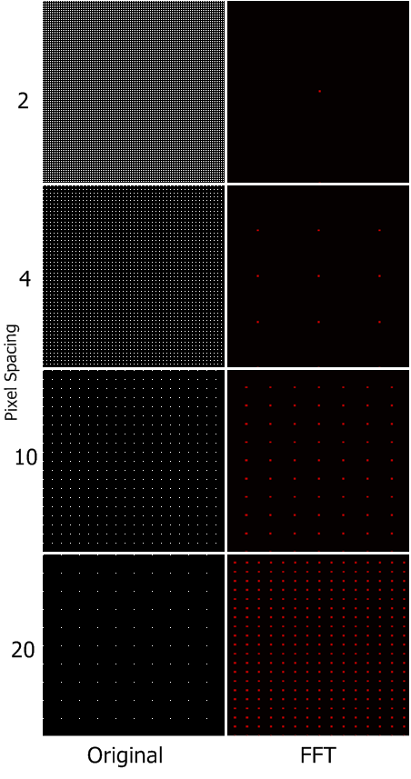
Figure 5. The effect of the pixel spacing in the FT domain.
We also try having only the x-axis and the y-axis with equally spaced ones. We see that the larger the spacing, the more ‘boxes’ appear. It is similar to that of Figure 4.
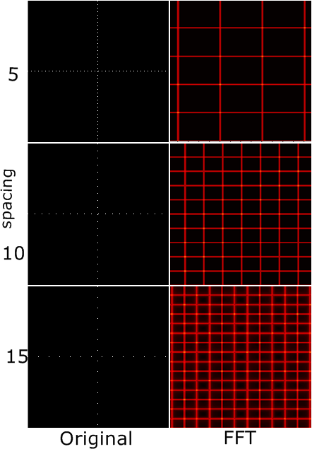
Figure 6. The effect of the pixel spacing in the x and y-axis in the FT domain.
Now we go to the more exciting part! We shall use FT to enhance images. First we use it on an image of the moon with lines. This is due to the fact that the whole image is a collection of images. Using Scilab, we first take the Fourier transform of the image. As you can see, on the y-axis are small dots. Those are the lines which we need to take out. We have used a mask to get rid of the peaks in the y-axis. I would like to acknowledge Ms. Krizia Lampa for the mask because she taught me how to use Photoshop in creating the mask! ;D I was really having a hard time doing it but thanks to her, I got to do it very fast. You just need to load the image in Photoshop, create a new layer, then with the pencil tool, blacken out the white pixels that you need to blacken out, hide the image of the FT, and put up a white background and voila! You have now your mask! You must now multiply the mask with the FT. Taking the inverse FT of the masked FFT will give you the enhanced image. It's the old image without the lines! 😄
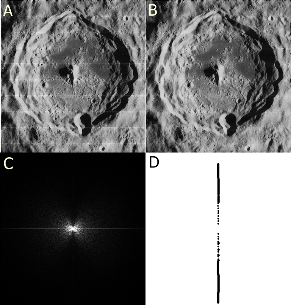
Figure 7. An image with recurring lines (a) was Fourier Transformed (c). A mask (d) was multiplied to the Fourier transform to remove the lines, creating (b).
We now try the same technique on a painting. We crop out a small portion of the painting and then try to remove the canvas weave patterns. As you can see, we have successfully removed the weave patterns! Yay! The strokes are seen better. 😄
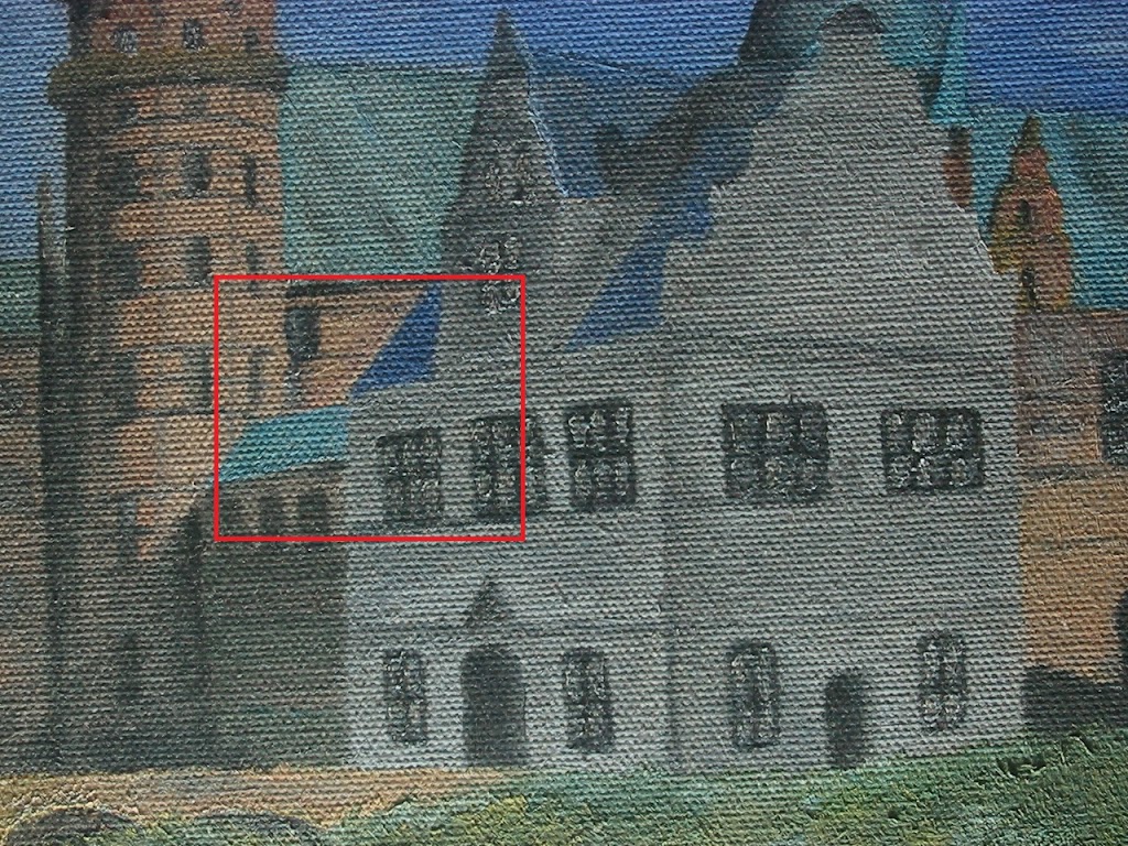
Figure 8. The painting used where the weave patterns are removed.
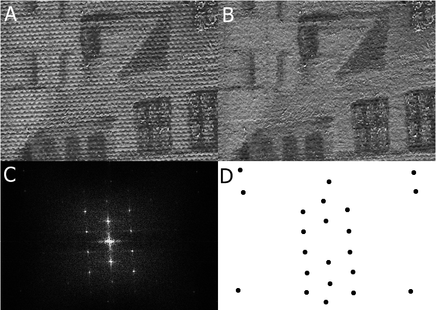
Figure 9. An image with weaving pattern (a) was Fourier Transformed (c). A mask (d) was multiplied to the Fourier transform to remove the weaving pattern, creating (b).
Lastly, we invert the filter mask in Figure 9b and then take its inverse Fourier transform. The result can be described as that of a circular aperture's FFT as seen in Figure 1. However, when you try to look closely, one can see ‘weave’ patterns. Amazing! 😄
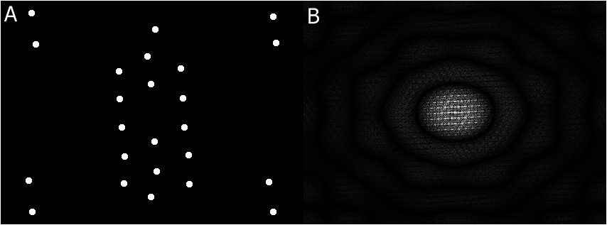
Figure 10. The inverted grayscale image of the mask in Figure 9b and its Fourier transform.
← All Image Processing articles