For the next activity, we used histogram manipulation for the enhancement of images. Well, why do we need it at all? Of course, not every picture is perfect. When I mean “perfect” (if in such case it exists), I may say that there may be flaws in the picture such as incorrect lighting or just the plain limitation of one's camera which makes it “imperfect”.
A picture can be characterized by the number of gray levels it has. In general, an image with good contrast (which is better!) has a uniform distribution of gray levels. Therefore, the image histogram must be a “flat” line covering the whole gray level scale. By manipulating the histogram of the image, we may be able to enhance its contrast.
A histogram of a grayscale image is equal to the graylevel probability distribution function (PDF) if normalized by the total number of pixels [1]. Using the PDF, we can calculate the cumulative distribution function (CDF) of the image. Using back projection of the original CDF to a desired CDF, one may improve the quality of an image. Figure 1 shows how back projection is done.
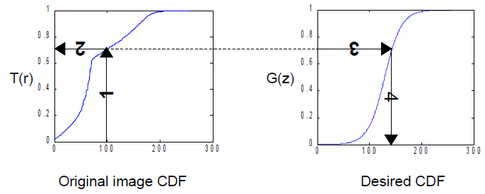
Figure 1. Steps in altering the grayscale distribution: (1) From pixel grayscale, find CDF value (2). Trace this value in the desired CDF (3). Replace pixel value by grayscale value having this CDF value in desired CDF (4). (Image and description taken from [1])
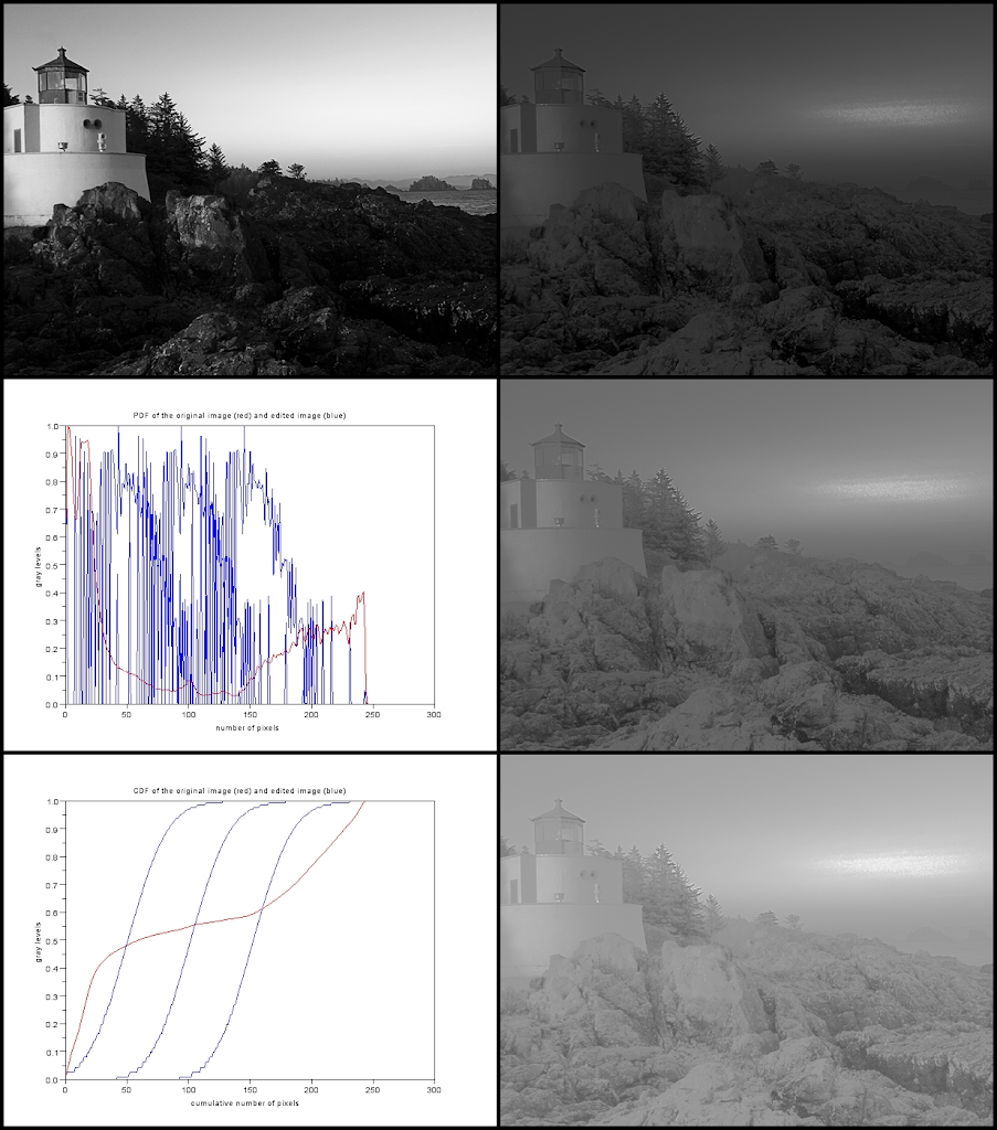
For this experiment, we have used the image of a lighthouse which was already installed in the Windows 7 operating system. It was turned into grayscale. The PDF was obtained and its CDF. As one may notice, the PDF is not flat and evenly distributed. This will be the image and the CDF that we shall use. Here are some code snippets I used:
Im = imread("E:\AP 186\Act 5\LH.jpg");
Im = rgb2gray(Im)
imwrite(Im, "E:\AP 186\Act 5\LH_gray.png");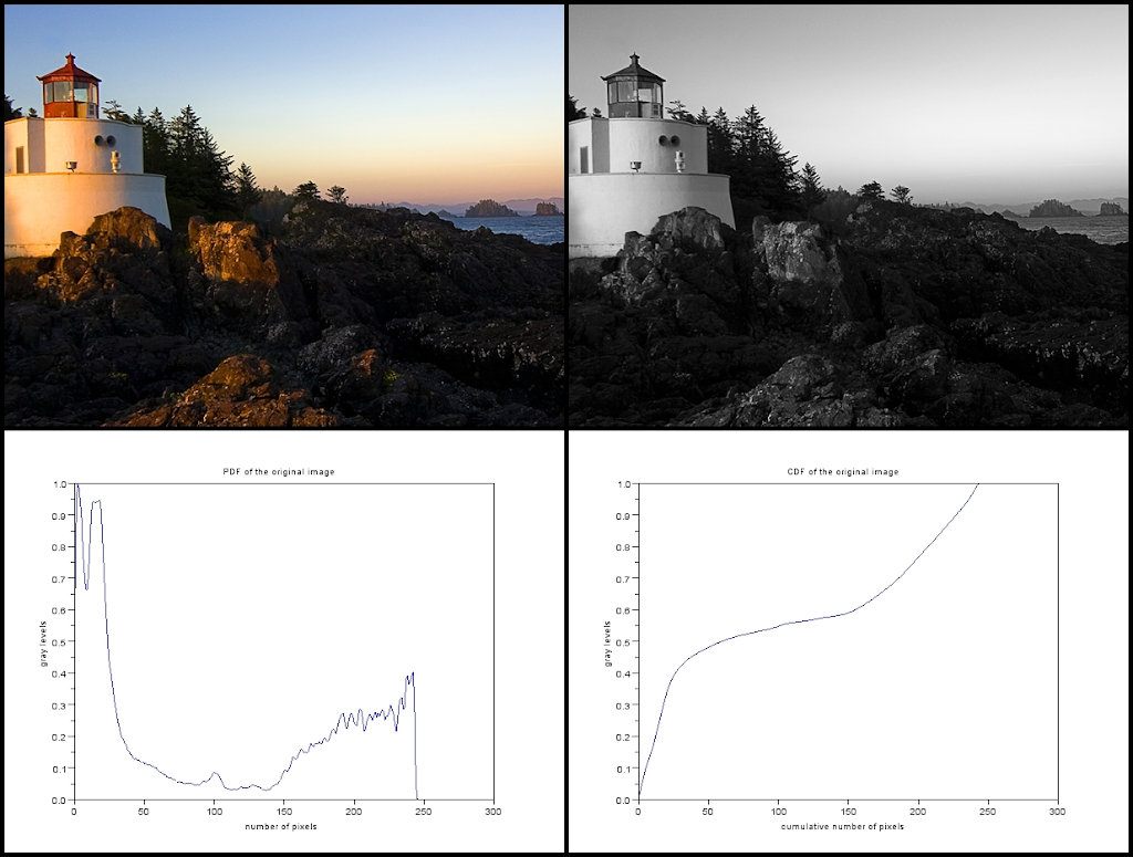
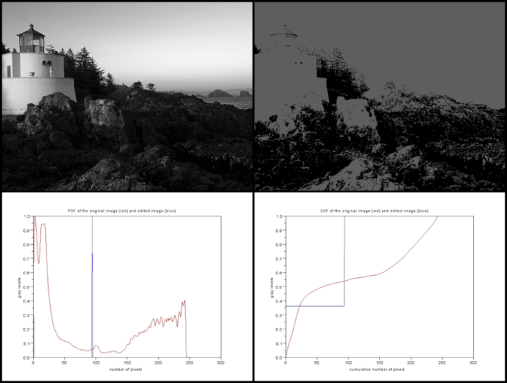
Figure 2. (Upper Left) The image of the lighthouse we shall be using. (Upper Right) The lighthouse in grayscale. (Lower Left) The PDF of the image. (Lower Right) The CDF of the image.
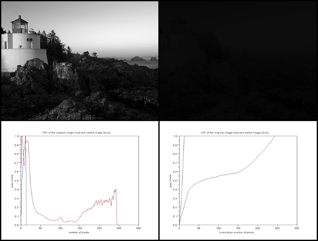
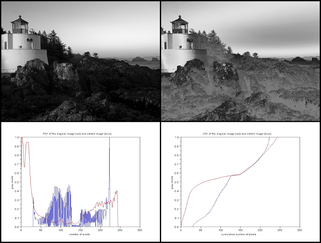
Now, what we shall do is back project the original's CDF to a desired CDF. I experimented with different kinds of “desired function”. First, I tried using a cube root function.
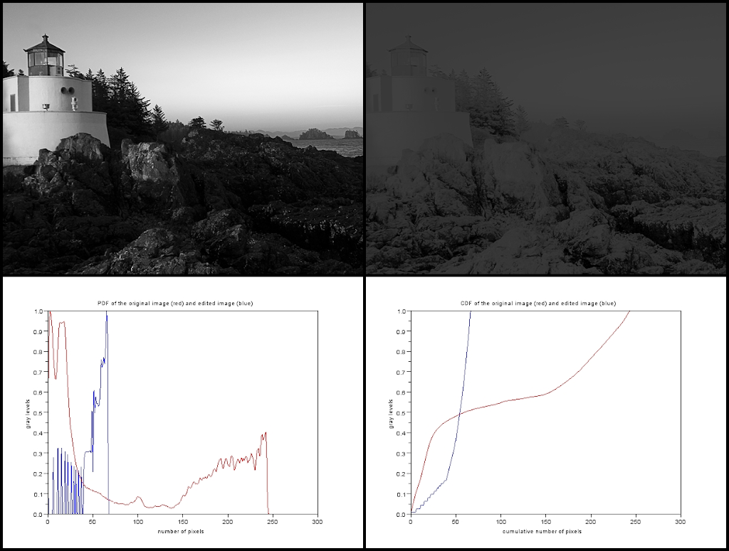
Figure 3. Cube root as the desired function. (Upper left) The original image. (Upper right) The manipulated image using the desired function. (Lower left) The PDF of the original image (red) and the PDF of the image after manipulation using the desired function. (Lower right) The CDF of the original image (red) and the CDF of the image after manipulation using the desired function.
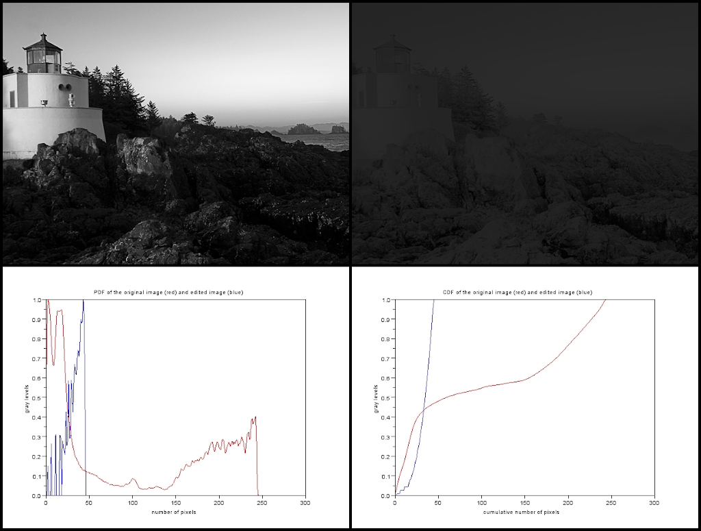
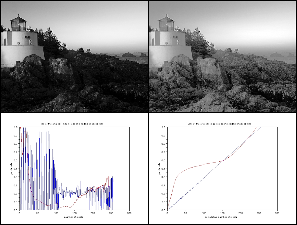
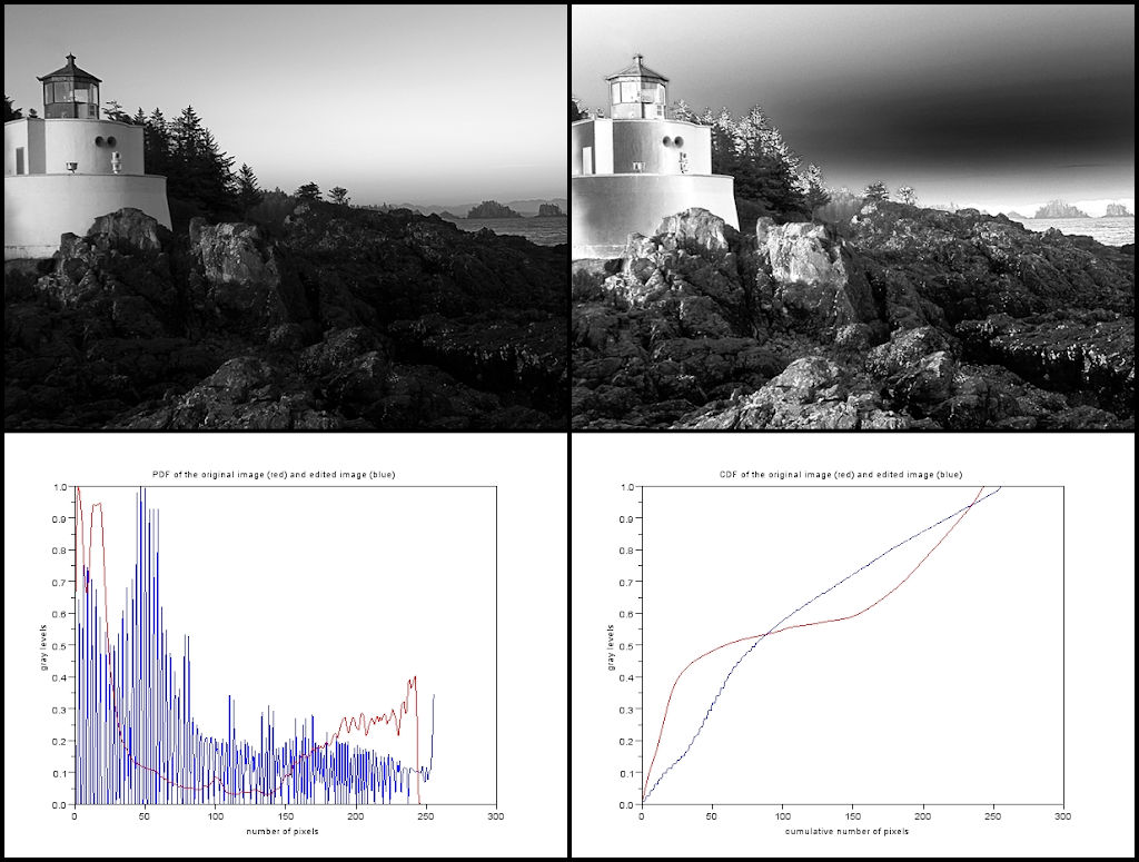
Oh! And it failed! As you can see from the PDF, the gray level distribution went to the left, making the image darker. Next I tried an exponential, squared and a square root function as my CDF.